Creo Simulate Day 1, Intro
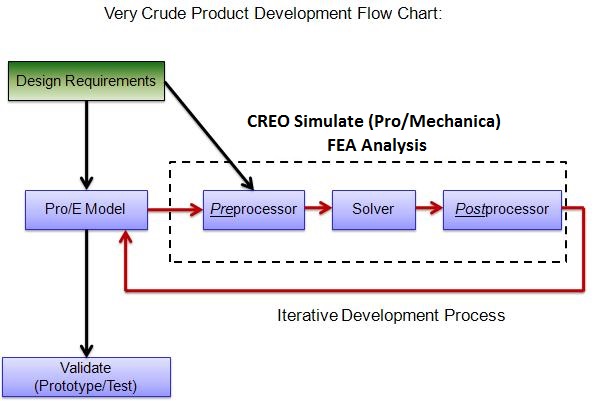
Overview: FEA workflow:
+ FEA (in general): + CREO Simulate:
– Pre-processor – Add loads / constraints and create P-mesh
– Solver – Run an analysis or design study
– Post processor – Review Results

To Start: Create a 24″ wide X 6″ high X 120″ long AL 6061 Cantilever Beam and go to ‘Applications’ then ‘Simulate’.
Pro Tip: Set the material in Creo Parametric before going into Simulate.
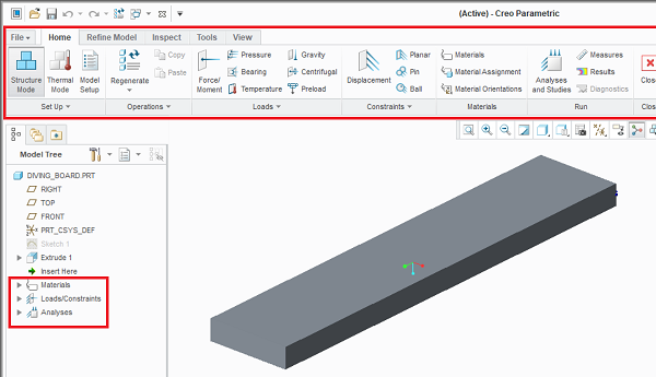
Let’s get familiar with the new dashboard ribbons and updated Model Tree.

Next: Setup the Static Structural Analysis.
- Constraint: Displacement=0 at the far end of the board
- Load: 250 lbs in the downwards direction at the near the end of the board
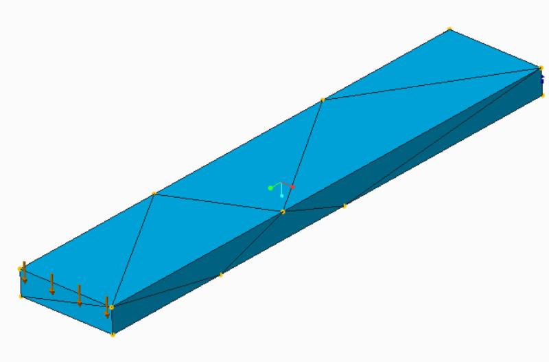
Next: Create the mesh using AutoGEM
Discuss:
- What is a mesh? What’s the difference between Nodes & Elements?
- ‘P-mesh’ and how it is utilized in Simulate
- High-order elements and why the software is performing iterations on a linear analysis
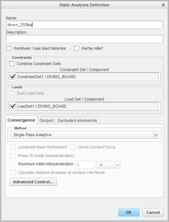
Next: Set up a new Static analysis like the one in the image to the left.
Pro Tip: Be sure to give the analysis a descriptive name!
Discuss: The differences between the 3 different convergence methods
- Quick check
- Single Pass Adaptive (SPA)
- Multi-Pass Adaptive (MPA)
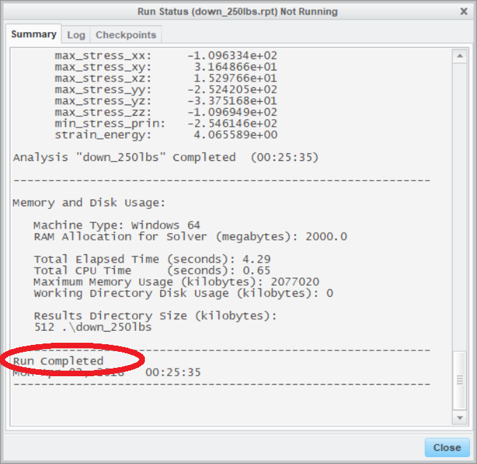
Next: Once the analysis is set up run it by clicking the green flag. Observe the run status to verify when the analysis is complete.

Next: View the results of your analysis.
Observe: The stress contour through the thickness of the part.
Explore:
- The post-processing tools: pictures, animations, and graphs
- Add another 250 lbs load in the -‘X’ direction and rerun the analysis. Add a mesh control to smooth out the stress plot
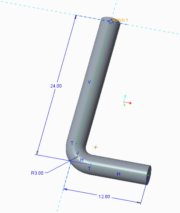
Next: Conduct a static analysis on this Nylon “Torsion Bar” using the same conditions as the previous analysis.
Notes:
- The diameter of the cross-section is 3.00
- Refine the mesh so the stress contour is smooth
Explore:
- Compare to the yield strength of nylon. Will the part fail?
- Change the 12″ long leg to 36″ and rerun the analysis. What’s different about the stress plot? What does this tell you about the possible failure mode?
- Increase the load 10X, and observe the new results. Were the results predictable? Is this good or bad? Is this realistic?

Next:
- Build a stainless steel column that is 5″ by 5″ by 20″
- Constrain the bottom to dx=dy=dz=0, and apply a 1,000 lbs vertical load in compression.
- After refining the mesh and verifying convergence, review the stress plot, and determine what happened
Try: Constrain the bottom utilizing edges or even vertices, to reduce the stress concentrations.
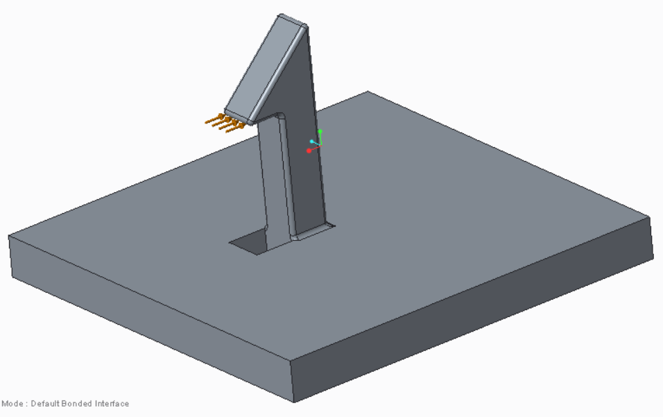
Next: Execute a static analysis on the linked model below. Constrain the bottom to d=0, and push the nylon clip inwards with a 10 lbs force.
- Conduct the analysis both with and without the radii on the model. What impact does this have on the mesh count?
- Review the stress and validate the accuracy by graphing the convergence. Smooth out the stress plot by adding mesh controls
- Instead of a force, push the clip in by 0.1″.
Download Model: Plastic_Clip
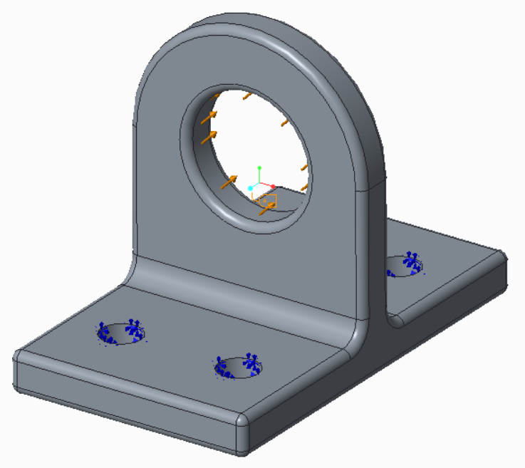
Next: Download the 6061 Aluminum lug model below, and prep for analysis; constrain the bottom surface to d=0, and put a 2,000 lbf force at a 45 degree angle as shown in the image. Verify convergence and review the stress.
Explore:
- Change the load to a bearing load and constrain the bolt pattern surfaces instead as it is more realistic. Compare the stress plots before and after
- Even more realistic is constraining the surface under the bolt head as this is the surface which actually constrains the lug. Utilize surface regions to isolate the bolt head footprint.
- Cut the model in half and rerun the analysis with a symmetry constraint. Are the results identical?
Model: Aluminum Lug
© Fastway Engineering. All Rights Reserved. May not be duplicated without express written consent.
